
Battery charge, health and anomaly#
The ESP-Mosaico has a small cell and a fuel gauge. OpenCarMind EdgeOS 2.1.0 estimates the cell’s state of charge and state of health, and checks it for faults. You see the results in plain words in the Health app. The fixed battery protection stays in charge of power: none of these models acts on it.
How the charge estimator works#
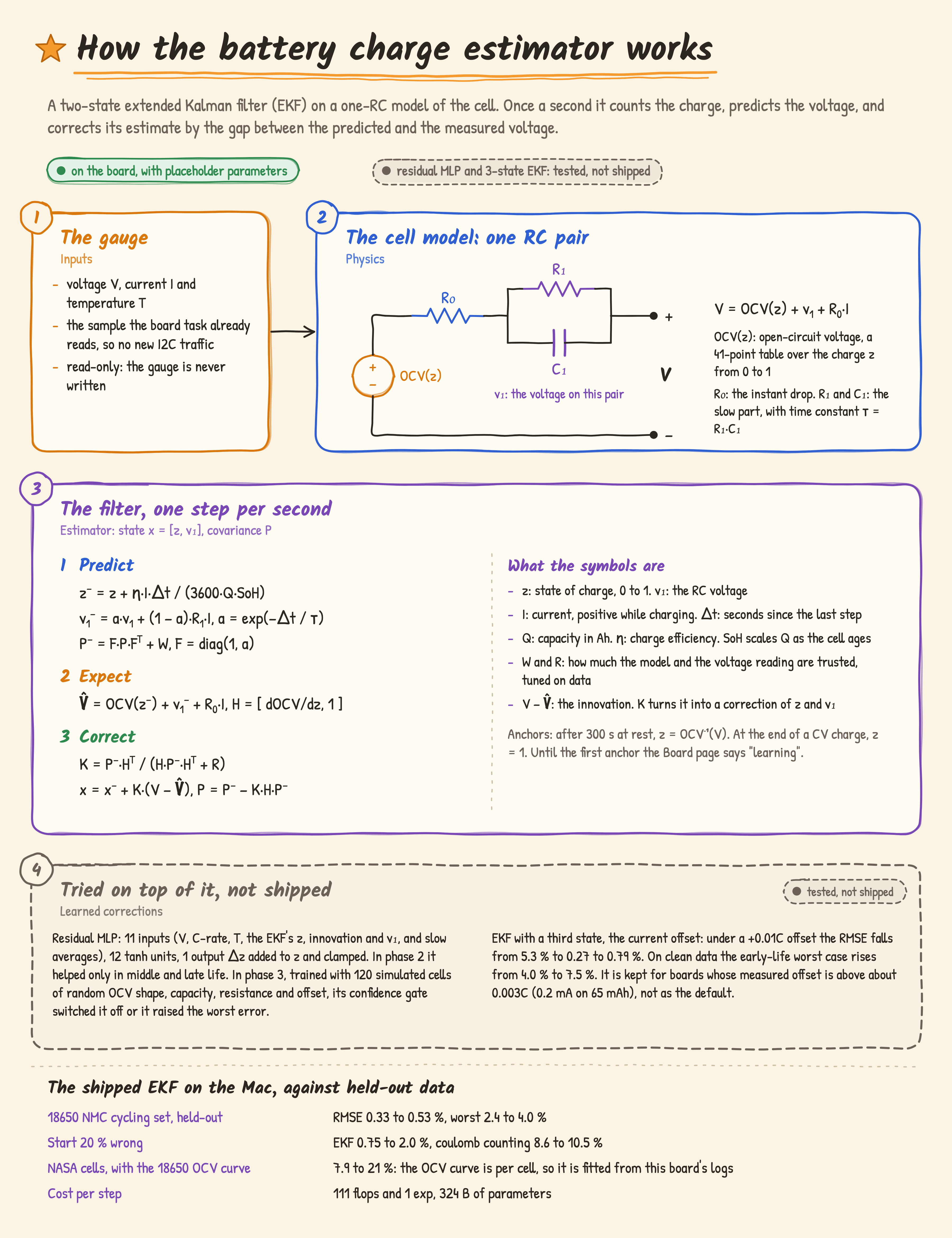
The cell is modelled as a voltage source that depends on the charge, OCV(z), in series with a resistance R₀ and one resistor-capacitor pair R₁ ∥ C₁. R₀ gives the instant drop when current flows. The RC pair gives the slow part, with time constant τ = R₁C₁. The filter keeps two states, the charge z (0 to 1) and the voltage v₁ on the RC pair, and a 2 × 2 covariance P that says how sure it is of them. Plett laid out this use of the extended Kalman filter for battery management systems[21].
Every second it predicts. It counts the charge and lets the RC voltage decay towards its new level:
Here I is the current in amps (positive while charging), Δt the seconds since the last step, Q the capacity in Ah, η the charge efficiency, and SoH the share of the capacity the cell still has. The covariance grows by the process noise W: P⁻ = F P Fᵀ + W, with F = diag(1, a).
Then it predicts the terminal voltage and compares it with the gauge:
The gap V − V̂ is the innovation. The Kalman gain K decides how much of it goes into each state:
R is the variance of the voltage reading. Where the OCV curve is steep, the voltage says a lot about z, and the filter follows it. Where the curve is flat, dOCV/dz is small, K shrinks, and the filter trusts the charge count. That is how a wrong start fixes itself: with the start 20 % off, the EKF’s error stayed at 0.75 to 2.0 % RMSE, where plain coulomb counting stayed at 8.6 to 10.5 %.
Two anchors reset the charge outright. After 300 s at rest the voltage is the OCV, so z = OCV⁻¹(V). At the end of a CV charge, z = 1. Until the first anchor the Board page says “learning”. Two anchors at least 30 % of charge apart give a capacity sample for the health estimate.
In the firmware (main/bat_est.c, math in main/bat_est_core.c, model in main/bat_model.h) the step matches the Mac reference to within 1.1e-6 over 370 test steps (make -C tests/host bat BAT_MODEL=<fitted header>). It reads the gauge sample the board task already takes every 2 s, so there is no new I2C traffic, and the gauge is never written. The learnt values and the last SoC go to NVS at most every 10 minutes and on the safe-shutdown path. Every 10 s a training row (V, I, average I, T, the gauge’s SoC and remaining capacity, the estimator’s SoC, SoH and mode) goes to obd/bat/bNNNNNN.csv on the NAND, at most 2 MB in all, oldest file first out. Those rows are what the cell’s own OCV curve will be fitted from. Until then the firmware runs placeholder parameters for a 4.2 V cell, and the nominal capacity is CONFIG_OCM_BAT_NOMINAL_MAH, 65 mAh from the cell’s label (UNVERIFIED).
Tested on the Mac, held out from fitting:
Test |
2-state EKF (shipped) |
For comparison |
|---|---|---|
An 18650 NMC cycling data set, held-out early, middle and late life |
RMSE 0.33 to 0.53 %, worst 2.4 to 4.0 % |
|
Start 20 % wrong |
RMSE 0.75 to 2.0 % |
coulomb counting 8.6 to 10.5 % |
NASA cells[26], with the 18650 cell’s OCV curve |
RMSE 7.9 to 21 % |
the OCV curve is specific to the cell, so it has to come from this board’s logs |
Current offset of +0.01C (0.65 mA on 65 mAh) |
RMSE 5.3 % |
the 3-state EKF: 0.27 to 0.79 % |
Cost per step |
111 flops and 1 exp, 324 B |
I checked where the EKF’s remaining error comes from. It is a slow drift of about ±0.3 % from counting charge, and it does not sit at the low-charge knee, in the CV taper or with heat. An unscented Kalman filter[22] with one or two RC pairs gave the same RMSE. Neither the linearisation nor the model order is the limit. The biggest risk is a current offset, which the 3-state EKF in the last dropdown is kept ready for.
How the health estimate works#
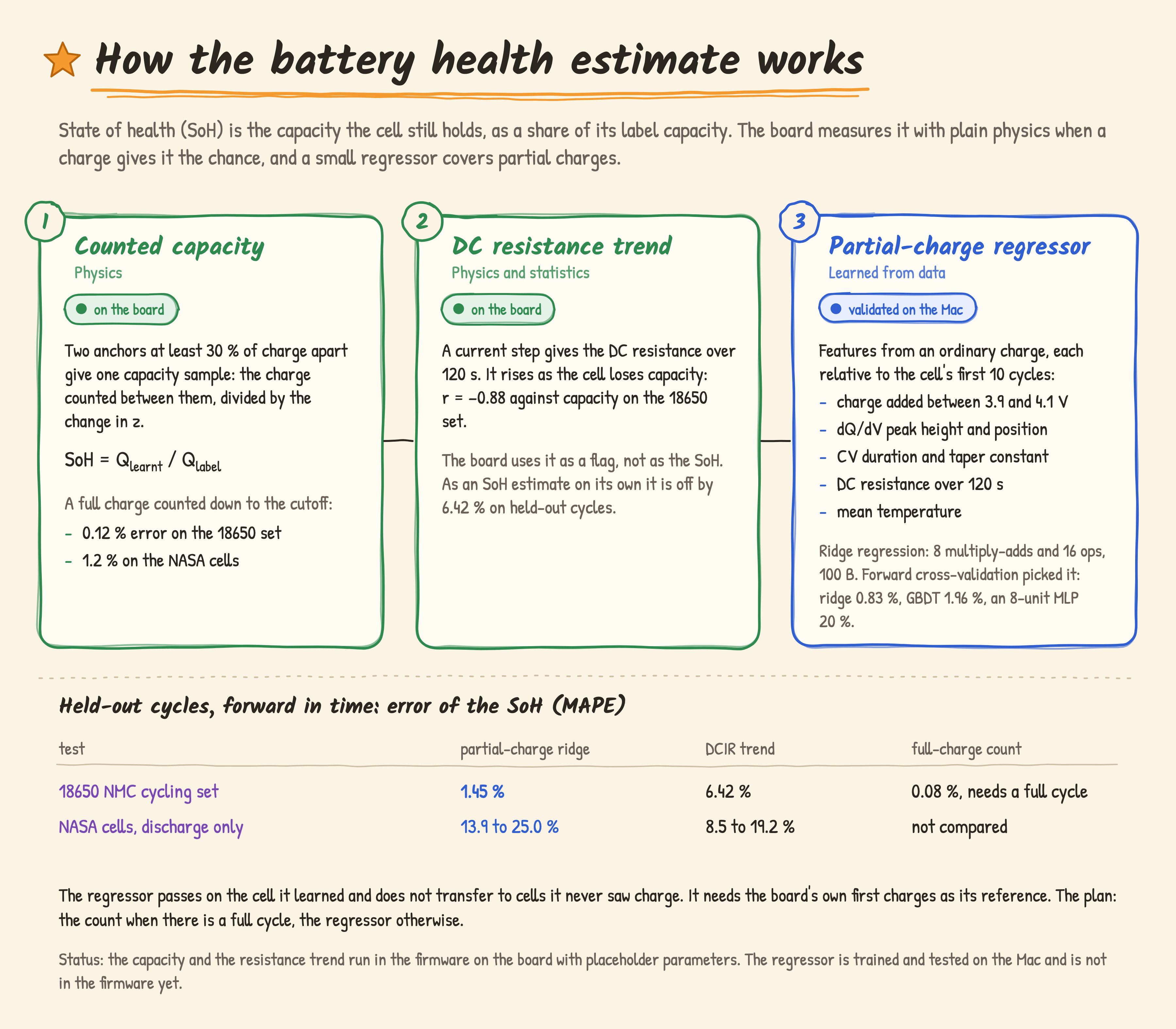
SoH is the capacity the cell still holds divided by its label capacity. The board gets it two ways.
The firmware counts it. Two anchors (a rest, or the end of a CV charge) at least 30 % of charge apart give one sample: the charge counted between them divided by the change in z. A full charge counted down to the cutoff was off by 0.12 % on the 18650 set and by 1.2 % on the NASA cells. Current steps also give a DC resistance (DCIR) over 120 s. It rises as the cell fades (r = −0.88 against capacity on the 18650 set), but as an SoH estimate on its own it is off by 6.42 %, so the board uses it as a flag.
A count from full to the cutoff needs the board to run its cell flat, which a board on the car’s USB rarely does. So I trained a regressor on what an ordinary charge shows. Its features are taken relative to the cell’s first 10 cycles: the charge added between 3.9 and 4.1 V, the height and position of the dQ/dV peak (the charge added per volt of rise), the CV duration and its taper constant, the DCIR over 120 s and the mean temperature. Ridge regression won the forward cross-validation (0.83 % against 1.96 % for a tree ensemble (GBDT) and 20 % for an 8-unit MLP). It costs 8 multiply-adds and 16 ops, in 100 B.
Held-out cycles, forward in time (MAPE) |
Partial-charge ridge |
DCIR trend |
Full-charge count |
|---|---|---|---|
18650 NMC cycling set |
1.45 % |
6.42 % |
0.08 %, needs a full cycle |
NASA cells[26], discharge only |
13.9 to 25.0 % |
8.5 to 19.2 % |
not compared |
The regressor passes on the cell it learned and does not transfer to cells it never saw charge. It needs the board’s own first charges as its reference. The plan is the count when there is a full cycle and the regressor otherwise. The regressor is in the firmware since 2.1.0, where its C matches the Mac to 1.3e-7. It has not run on the board yet: it needs 10 deep charges of this cell as its reference, and in the 2.1.0 board check the cell stayed full (0 of 10).
How the anomaly detector works#
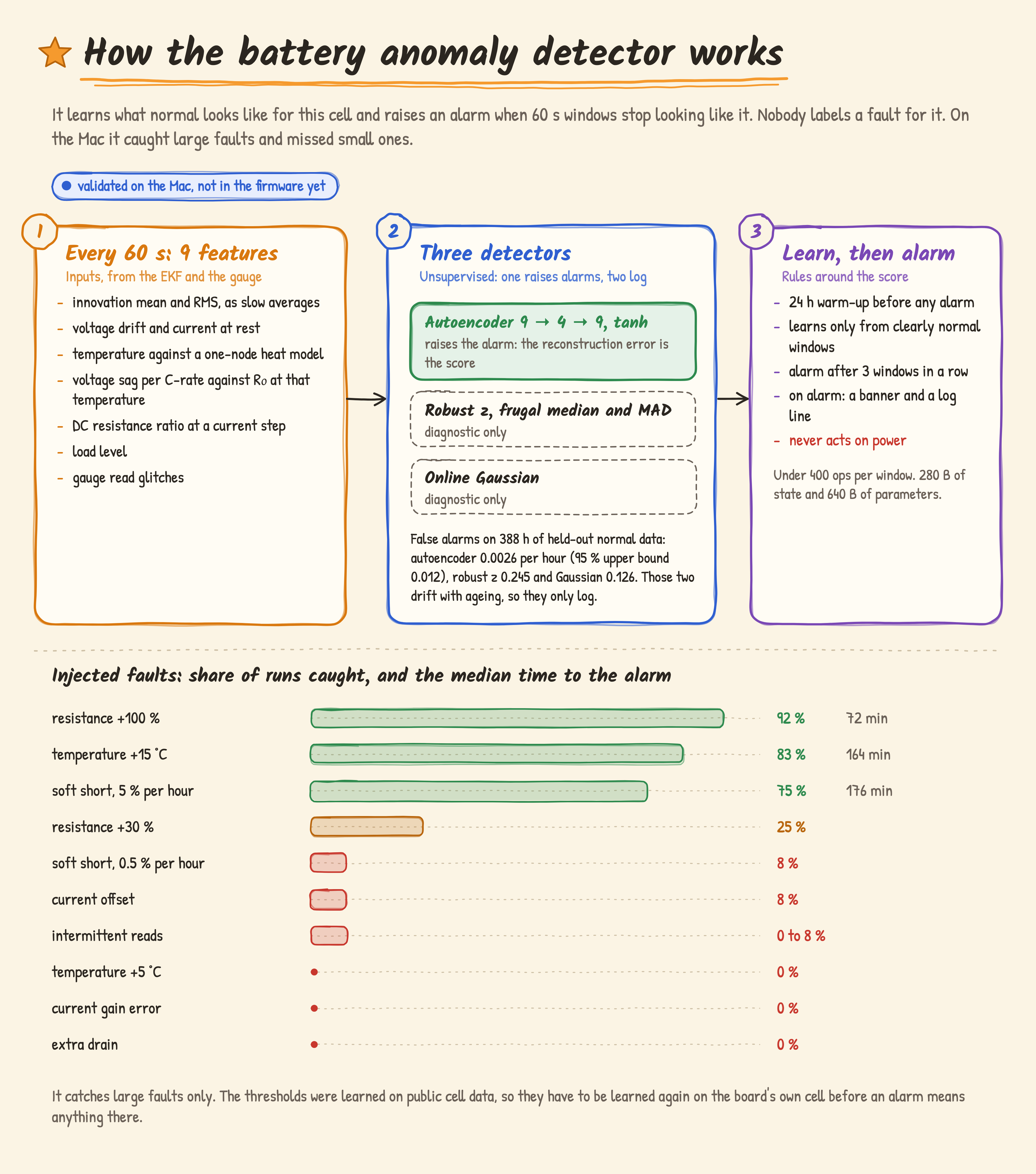
The detector learns what normal looks like for this cell and raises an alarm when 60 s windows stop looking like it. Nobody labels a fault for it. Each window has 9 features from the EKF and the gauge: the innovation’s mean and RMS as slow averages, the voltage drift and the current at rest, the temperature against a one-node heat model, the voltage sag per C-rate against R₀ at that temperature, the DC resistance ratio at a current step, the load level and the gauge’s read glitches.
Three detectors ran side by side. One is a z-score against a frugal streaming median and MAD[25], one an online Gaussian, and one a 9 → 4 → 9 tanh autoencoder whose score is its reconstruction error. All three warm up for 24 h, learn only from clearly normal windows, and alarm after 3 windows in a row. On 388 h of held-out normal data the autoencoder gave 0.0026 false alarms per hour (95 % upper bound 0.012). The z-score gave 0.245 per hour and the Gaussian 0.126, because the cell’s ageing moved them. So only the autoencoder raises alarms, and the other two only log.
Injected fault |
Caught |
Median time to the alarm |
|---|---|---|
Resistance +100 % |
92 % |
72 min |
Temperature +15 °C |
83 % |
164 min |
Soft short, 5 % of capacity per hour |
75 % |
176 min |
Resistance +30 % |
25 % |
|
Soft short, 0.5 % per hour |
8 % |
|
Current offset |
8 % |
|
Intermittent reads |
0 to 8 % |
|
Temperature +5 °C, current gain error, extra drain |
0 % |
It catches large faults only. The thresholds were learned on public cell data, so they have to be learned again on the board’s own cell before an alarm means anything there. An alarm shows a banner and writes a log line. It never acts on power: the fixed battery protection above stays in charge of that. The cost is under 400 ops a window, with 280 B of state and 640 B of parameters. It is in the firmware since 2.1.0, within 1.05e-6 of the Mac, and the 2.1.0 board check admitted it and started its 24 h warm-up. A real fault has not been seen in use yet. The worn and fault cards shown so far come from a test build that writes a state into the Health screen only.
The status of each model on the board is in the table on AI services.